How to make AI-powered forecasts in Apache Superset and Snowflake using MindsDB
How to make AI-powered forecasts in Apache Superset and Snowflake using MindsDB

Martyna Slawinska, Technical Product Manager at MindsDB
Oct 27, 2021

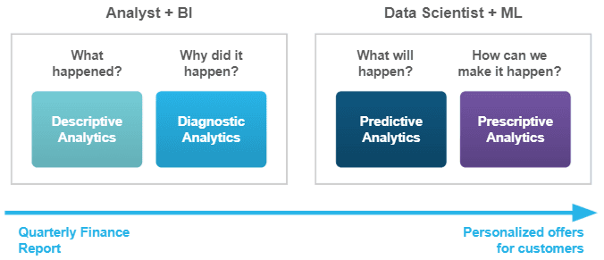
There is an ongoing transformational shift within the modern business world from the "what happened and why" based on historical data analysis to the "what will we predict can happen and how can we make it happen" based on machine learning predictive modeling.
The success of your predictions depends both on the data you have available and the models you train this data on. Data Scientists and Data Engineers need best-in-class tools to prepare the data for feature engineering, the best training models, and the best way of deploying, monitoring, and managing these implementations for optimal prediction confidence.
Running MindsDB with Snowflake can significantly increase the performance and reduce the computational requirements of training your machine learning models. If you are already a Snowflake user, you can take advantage of key features quickly to enable fast, efficient machine learning capabilities directly in your database by simply connecting Snowflake to the MindsDB service.
In this article, we will show you how to connect Snowflake to MindsDB, how you can enable real-time machine learning with Snowflake and MindsDB, and how to visualize the MindsDB predictions with Apache Superset.
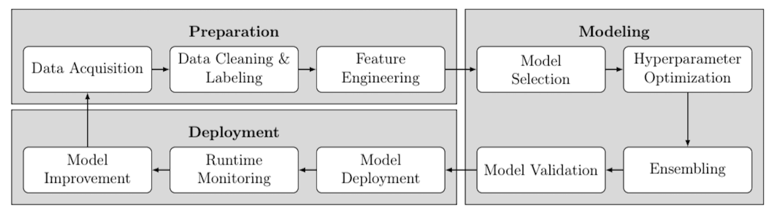
Machine Learning (ML) Lifecycle
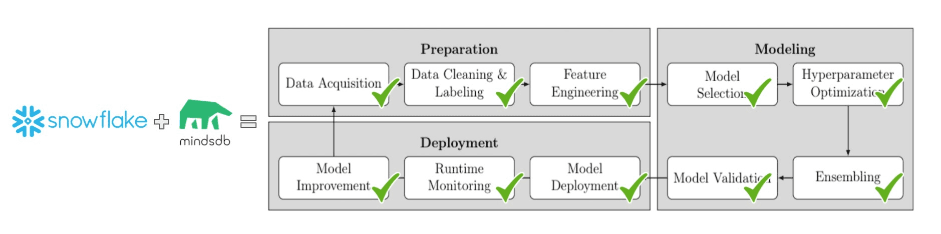
The ML lifecycle can be represented as a process that consists of the data preparation phase, modeling phase, and deployment phase. The diagram below presents all the steps included in each of the stages.
Companies looking to implement machine learning have found their current solutions require substantial amounts of data preparation, cleaning, and labeling, plus hard to find machine learning/AI data scientists to conduct feature engineering; build, train, and optimize models; assemble, verify, and deploy into production; and then monitor in real-time, improve, and refine. Machine learning models require multiple iterations with existing data to train. Additionally, extracting, transforming, and loading (ETL) data from one system to another is complicated, leads to multiple copies of information, and is a compliance and tracking nightmare.
A recent study has shown it takes 64% of companies a month, to over a year, to deploy a machine learning model into production¹. Leveraging existing databases and automating the feature engineering, building, training, and optimization of models, assembling them, and deploying them into production is called AutoML and has been gaining traction within enterprises for enabling non-experts to use machine learning models for practical applications.
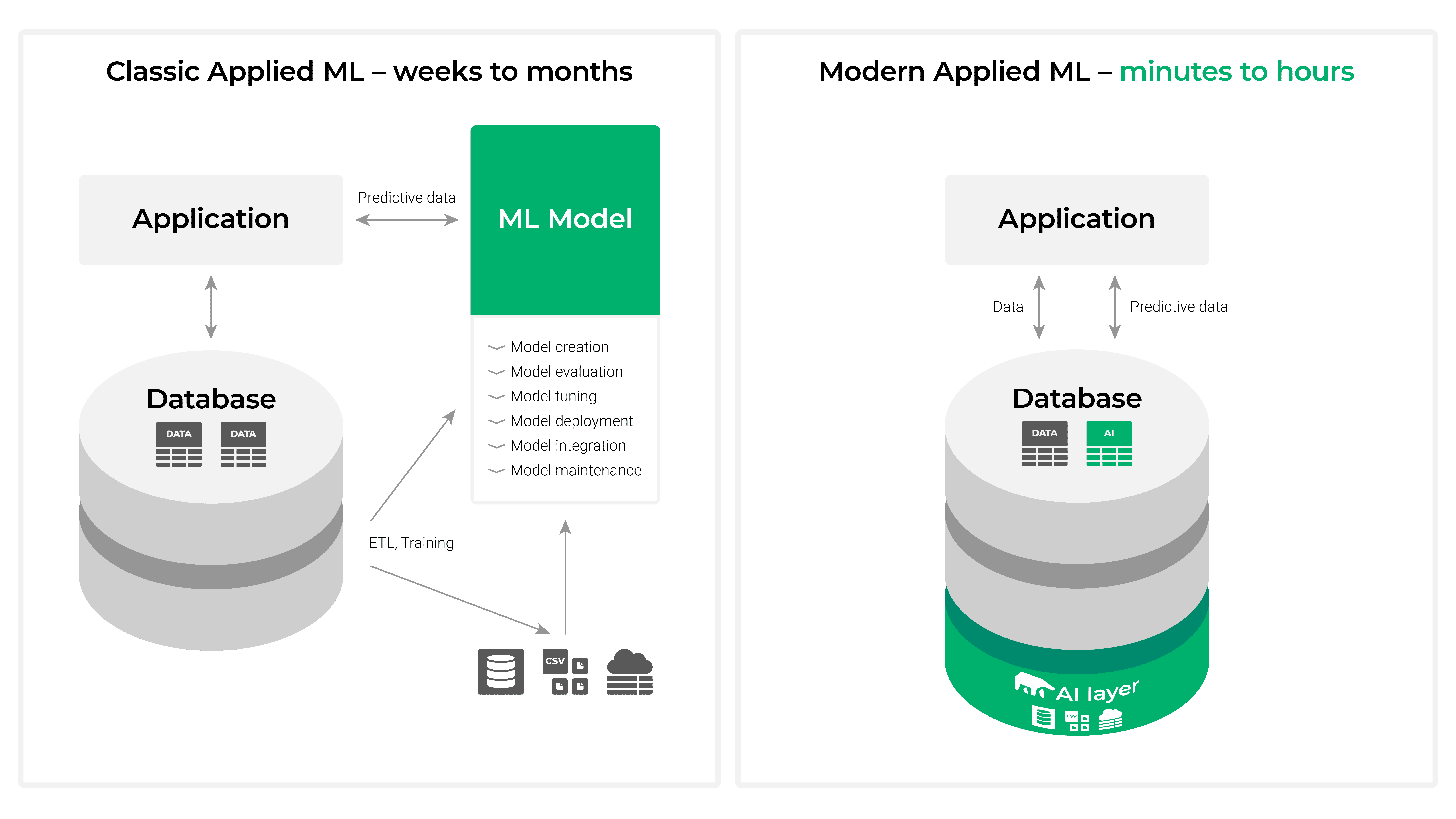
MindsDB brings machine learning to existing SQL databases with a concept called AI Tables. AI Tables integrate the machine learning models as virtual tables inside a database, create predictions, and can be queried with simple SQL statements. Almost instantly, time series, regression, and classification predictions can be done directly in your database.
Deep Dive into the AI Tables
Let’s consider the following income table that stores the income and debt values.
SELECT income, debt FROM
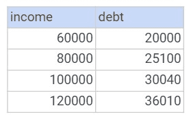
A simple visualization of the data present in the income table is as follows.
Querying the income table to get the debt value for a particular income value results in the following.
SELECT income, debt FROM income
WHERE income = 80000

But what happens when we query the table for income value that is not present?
SELECT income, debt FROM income
WHERE income = 90000
When a table doesn’t have an exact match the query will return a null value. This is where the AI Tables come into play!
Let’s create a debt model that allows us to approximate the debt value for any income value. We’ll train this debt model using the income table’s data.
CREATE MODEL debt_model
TRAIN FROM
MindsDB provides the CREATE MODEL statement. When we execute this statement, the predictive model works in the background, automatically creating a vector representation of the data that can be visualized as follows.
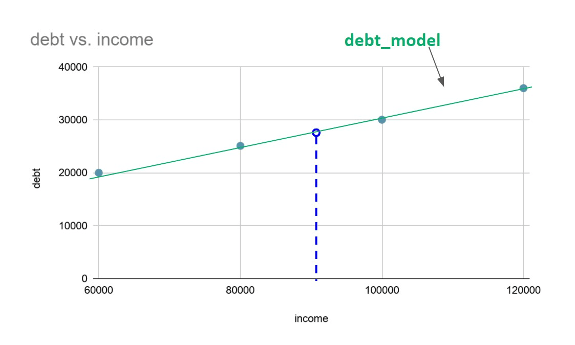
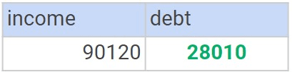
Let’s now look for the debt value of some random income value. To get the approximated debt value, we query the debt_model and not the income table.
SELECT income, debt FROM debt_model
WHERE income = 90120
Using MindsDB Machine Learning to Solve a Real-World Problem
Now, let’s use these powerful AI tables in a real-world scenario.
Imagine that you are a data analyst at the Chicago Transit Authority. Every day, you need to optimize the number of buses per route to avoid overcrowded or empty buses. You need machine learning to forecast the number of rides per bus, per route, and by time of day. The data you have looks like the table below with route_id, timestamp, number of rides, and day-type (W = weekend)
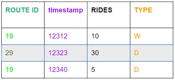
This is a difficult machine learning problem that is common in databases. A timestamp indicates that we are dealing with the time-series problem. The data is further complicated by the type of day (day-type) the row contains and this is called multivariate. Additionally, there is high-cardinality as each route will have multiple row entries each with different timestamps, rides, and day types.
Let’s see how we can use machine learning with MindsDB to optimize the number of buses per route and visualize the results.
Set Up MindsDB
First things first! You need to connect your database to MindsDB. One of the easy ways to do so is to to deploy MindsDB locally, please refer to installation instructions via Docker, MindsDB’s Extension on Docker Desktop or AWS Marketplace.
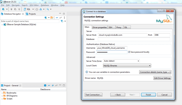
Once an account is created you can connect to Snowflake using standard parameters like database name (in this case the Chicago Transit Authority), host, port, username, password, etc.

Connect MindsDB to the Data for model training
MindsDB works through a MySQL Wire protocol. Therefore, you can connect to it using any MySQL client. Here, we’ll use the DBeaver database client and can see the Snowflake databases we are connected to.
Step 1: Getting the Training Data
We start by getting the training data from the database that we connected to our MindsDB cloud account. It is always good to first make sure that all the databases are present and the connections correct.
MindsDB comes with some built-in databases as follows:
INFORMATION_SCHEMA stores information about MindsDB,
MINDSDB stores metadata about the predictors and allows access to the created predictors as tables,
DATASOURCE for connecting to data or uploading files.
The SNF database is the database of the Chicago Transit Authority that we connected. It provides us with the training data. Let’s check it.
use snf;
SELECT *
FROM CHICAGO_TRANSIT_AUTHORITY.PUBLIC.CTA_BUS_RIDES_LATEST
LIMIT 100
The training data consists of the number of rides per bus route and day. For example, on 2001-07-03, there were 7354 rides on bus route 3.
Step 2: Training the Predictive Model
Let’s move on to the next step, which is training the predictive model. For that, we’ll use the MINDSDB database.
MINDSDB database comes with the predictors and commands tables. The predictors table lets us see the status of our predictive models. For example, assuming that we have already trained our predictive model for forecasting the number of rides, we’ll see the following.
SELECT name, status FROM
The process of training a predictive model using MindsDB is as simple as creating a view or a table.
CREATE MODEL rides_forecaster_demo FROM snf (
SELECT ROUTE, RIDES, DATE
FROM CHICAGO_TRANSIT_AUTHORITY.PUBLIC.CTA_BUS_RIDES_LATEST
WHERE DATE > '2020-01-01'
) PREDICT RIDES
ORDER BY DATE
GROUP BY ROUTE
WINDOW 10
HORIZON 7
Let’s discuss the statement above. We create a predictor table using the CREATE PREDICTOR statement and specifying the database from which the training data comes.
The code in yellow selects the filtered training data. After that, we use the PREDICT keyword to define the column whose data we want to forecast.
Next, there are standard SQL clauses, such as ORDER BY, GROUP BY, WINDOW, and HORIZON. We use the ORDER BY clause and the DATE column as its argument. By doing so, we emphasize that we deal with a time-series problem. We order the rows by date. The GROUP BY clause divides the data into partitions. Here, each of them relates to a particular bus route. We take into account just the last ten rows for every given prediction. Hence, we use WINDOW 10. To prepare the forecast of the number of bus rides for the next week, we define HORIZON 7.
Now, you can execute the CREATE PREDICTOR statement and wait until your predictive model is complete. The MINDSDB.PREDICTORS table stores its name as rides_forecaster_demo and its status as training. Once your predictive model is ready, the status changes to complete.
Step 3: Getting the Forecasts
We are ready to go to the last step, i.e., using the predictive model to get future data. One way is to query the rides_forecaster_demo predictive model directly. Another way is to join this predictive model table to the table with historical data before querying it.
We consider a time-series problem. Therefore, it is better to join our predictive model table to the table with historical data.
SELECT tb.ROUTE, tb.RIDES AS PREDICTED_RIDES
FROM snf.PUBLIC.CTA_BUS_RIDES_LATEST AS ta
JOIN mindsdb.rides_forecaster_demo AS tb
WHERE ta.ROUTE = "171" AND ta.DATE > LATEST
LIMIT 7
Let’s analyze it. We join the table that stores historical data (i.e., snf.PUBLIC.CTA_BUS_RIDES_LATEST) to our predictive model table (i.e., mindsdb.rides_forecaster_demo). The queried information is the route and the predicted number of rides per route. And the usage of the condition ta.DATE > LATEST (provided by MindsDB) ensures that we get the future number of rides per route.
Let’s run the query above to forecast the number of rides for route 171 in the next seven days.
Now we know the number of rides for route 171 in the next seven days. We could do it in the same way for all the other routes.
Thanks to the special SQL syntax that includes CREATE PREDICTOR, PREDICT, and > LATEST, MindsDB makes it straightforward to run predictors on our chosen data.
Now, let’s visualize our predictions.
Visualizing the Results using Apache Superset
Apache Superset is a modern, open-source data exploration and visualization platform designed for all data personas in an organization. Superset ships with a powerful SQL editor and a no-code chart builder experience. Superset ships with support for most SQL databases out of the box and over 50 visualization types.
You can connect to the Snowflake database or your MindsDB database that has a Snowflake connection within. Upon starting up your Superset workspace, your earlier defined database connection is ready to use! So you have access to the Chicago Transit Authority data, as well as to the predictions made by MindsDB.
Visualizing Data
The two data sets that we are relevant for visualization are the stops_by_route and forecasts data sets. The stops_by_route data set contains the exact location of each bus stop for each bus route. And the forecasts data set stores the actual and predicted number of rides, confidence interval, and lower and upper bounds of prediction, per route and timestamp.
Superset lets us visualize the stops_by_route data set as follows.
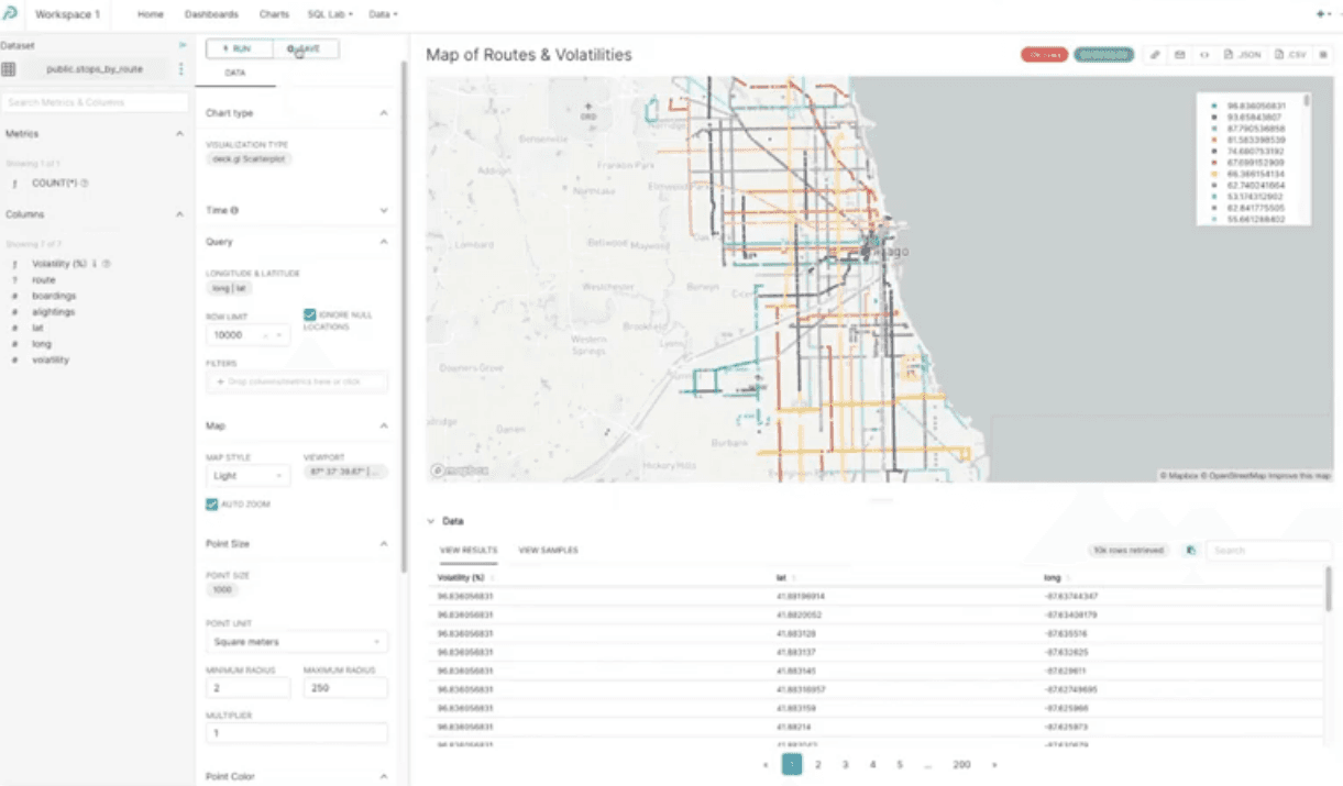
Every bus route has a different color. Also, there is volatility associated with each bus route. Let’s publish this chart to a new dashboard by clicking the +Save button, then switch to the Save as tab, and then type in “Routes Dashboard” in the Add to Dashboard field.
Now, let’s craft a time-series line chart to visualize actual vs predicted riders. Let’s look at the chart that presents the actual number of bus riders (in blue) and the predicted number of bus rides (in purple).
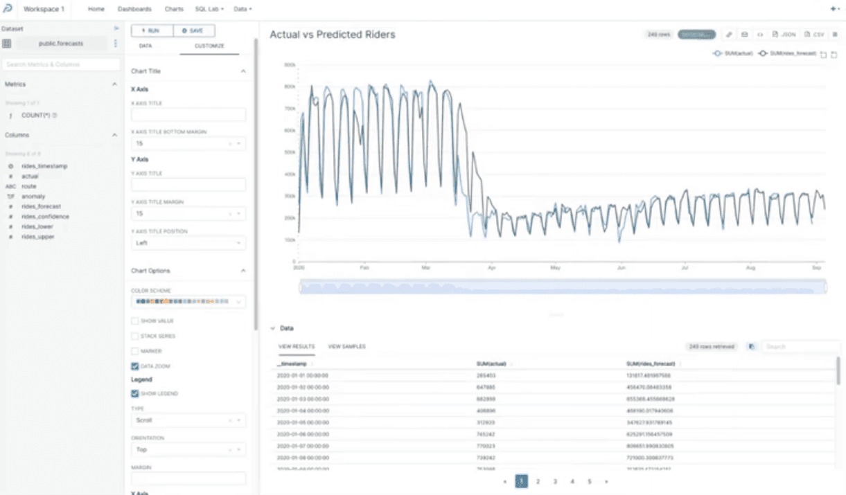
Predictions made by MindsDB closely resemble the actual data, except for a short time during March 2020 when the large-scale lockdowns took place. There we see a sudden drop in the number of bus rides. But MindsDB took some time to cope with this new reality and adjust its predictions.
Lastly, let’s add a data zoom to this chart for end-users to zoom in on specific date ranges. Click the Customize tab and then click Data Zoom to enable it. Then, click the + Save button and publish to the same “Routes Dashboard”.
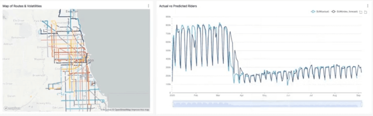
Let’s head over to the dashboard now and customize it to make it more dynamic and explorable. Click Dashboards in the top nav bar and then select “Routes Dashboard” from the list of dashboards. You can rearrange the chart positions by clicking the pencil icon, dragging the corners of the chart objects, and then clicking Save.
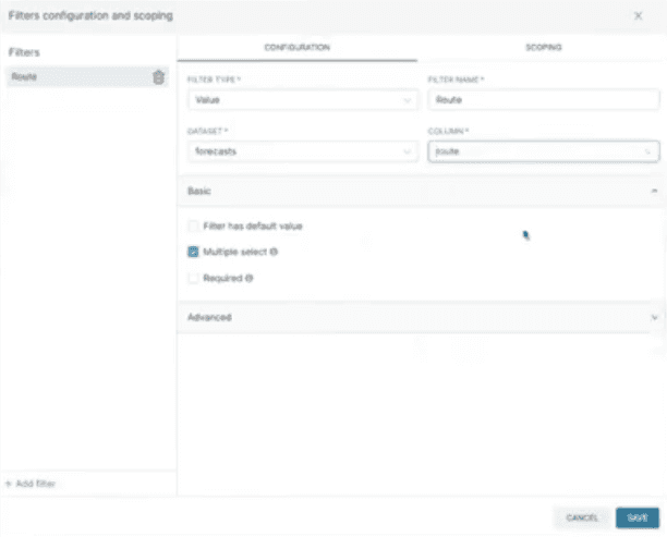
Let’s add some dashboard filters to this dashboard so dashboard consumers can filter the charts down to specific bus routes and volatility values. Click the right arrow (->) to pop open the filter tray. Then select the pencil icon to start editing this dashboard’s filters. Create the following filters with appropriate filter names:
A Value filter on the route column from the forecasts table.
A Numerical range filter on the volatility column from the stops_by_route table.
Click Save to publish these filters.
Let’s give these filters for a test ride! Use the routes filter to only show information for routes 1, 100, and 1001.
We could zoom in to see the time during the first large-scale lockdowns in March 2020. For these particular routes, the predictions made by MindsDB are not so far off.
Now, let’s use our volatility filter to view only the routes with volatility values greater than 55.
MindsDB does a pretty good job as the actual and predicted number of rides are pretty close!
Conclusions: Powerful forecasting with MindsDB, Snowflake, and Superset
The combination of MindsDB and Snowflake covers all the phases of the ML lifecycle. And Superset helps you to visualize the data in any form of diagrams, charts, or dashboards.
MindsDB provides easy-to-use predictive models through AI Tables. You can create these predictive models using SQL statements and feeding the input data. Also, you can query them the same way you query a table. The easiest way to get started with Superset is with the free tier for Preset Cloud, a hassle-free and fully hosted cloud service for Superset.
Want to try it out yourself?
Bookmark MindsDB repository on GitHub
Access MindsDB via Docker, MindsDB’s Extension on Docker Desktop or AWS Marketplace.
Engage with the MindsDB community on Slack or GitHub to ask questions, share and express ideas and thoughts.
If this article was helpful, please give us a GitHub star here.
References:
¹ Data adapted from Algorithmia (2021). 2021 state of enterprise machine learning.
There is an ongoing transformational shift within the modern business world from the "what happened and why" based on historical data analysis to the "what will we predict can happen and how can we make it happen" based on machine learning predictive modeling.
The success of your predictions depends both on the data you have available and the models you train this data on. Data Scientists and Data Engineers need best-in-class tools to prepare the data for feature engineering, the best training models, and the best way of deploying, monitoring, and managing these implementations for optimal prediction confidence.
Running MindsDB with Snowflake can significantly increase the performance and reduce the computational requirements of training your machine learning models. If you are already a Snowflake user, you can take advantage of key features quickly to enable fast, efficient machine learning capabilities directly in your database by simply connecting Snowflake to the MindsDB service.
In this article, we will show you how to connect Snowflake to MindsDB, how you can enable real-time machine learning with Snowflake and MindsDB, and how to visualize the MindsDB predictions with Apache Superset.
Machine Learning (ML) Lifecycle
The ML lifecycle can be represented as a process that consists of the data preparation phase, modeling phase, and deployment phase. The diagram below presents all the steps included in each of the stages.
Companies looking to implement machine learning have found their current solutions require substantial amounts of data preparation, cleaning, and labeling, plus hard to find machine learning/AI data scientists to conduct feature engineering; build, train, and optimize models; assemble, verify, and deploy into production; and then monitor in real-time, improve, and refine. Machine learning models require multiple iterations with existing data to train. Additionally, extracting, transforming, and loading (ETL) data from one system to another is complicated, leads to multiple copies of information, and is a compliance and tracking nightmare.
A recent study has shown it takes 64% of companies a month, to over a year, to deploy a machine learning model into production¹. Leveraging existing databases and automating the feature engineering, building, training, and optimization of models, assembling them, and deploying them into production is called AutoML and has been gaining traction within enterprises for enabling non-experts to use machine learning models for practical applications.
MindsDB brings machine learning to existing SQL databases with a concept called AI Tables. AI Tables integrate the machine learning models as virtual tables inside a database, create predictions, and can be queried with simple SQL statements. Almost instantly, time series, regression, and classification predictions can be done directly in your database.
Deep Dive into the AI Tables
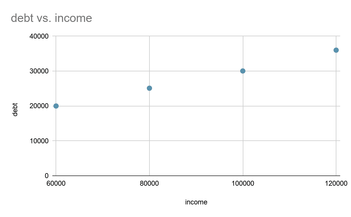
Let’s consider the following income table that stores the income and debt values.
SELECT income, debt FROM
A simple visualization of the data present in the income table is as follows.
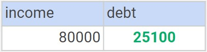
Querying the income table to get the debt value for a particular income value results in the following.
SELECT income, debt FROM income
WHERE income = 80000
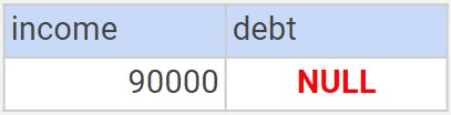
But what happens when we query the table for income value that is not present?
SELECT income, debt FROM income
WHERE income = 90000
When a table doesn’t have an exact match the query will return a null value. This is where the AI Tables come into play!
Let’s create a debt model that allows us to approximate the debt value for any income value. We’ll train this debt model using the income table’s data.
CREATE MODEL debt_model
TRAIN FROM
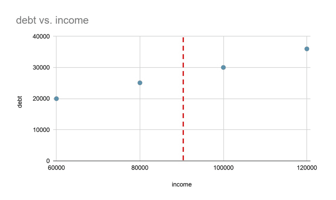
MindsDB provides the CREATE MODEL statement. When we execute this statement, the predictive model works in the background, automatically creating a vector representation of the data that can be visualized as follows.
Let’s now look for the debt value of some random income value. To get the approximated debt value, we query the debt_model and not the income table.
SELECT income, debt FROM debt_model
WHERE income = 90120
Using MindsDB Machine Learning to Solve a Real-World Problem
Now, let’s use these powerful AI tables in a real-world scenario.
Imagine that you are a data analyst at the Chicago Transit Authority. Every day, you need to optimize the number of buses per route to avoid overcrowded or empty buses. You need machine learning to forecast the number of rides per bus, per route, and by time of day. The data you have looks like the table below with route_id, timestamp, number of rides, and day-type (W = weekend)
This is a difficult machine learning problem that is common in databases. A timestamp indicates that we are dealing with the time-series problem. The data is further complicated by the type of day (day-type) the row contains and this is called multivariate. Additionally, there is high-cardinality as each route will have multiple row entries each with different timestamps, rides, and day types.
Let’s see how we can use machine learning with MindsDB to optimize the number of buses per route and visualize the results.
Set Up MindsDB
First things first! You need to connect your database to MindsDB. One of the easy ways to do so is to to deploy MindsDB locally, please refer to installation instructions via Docker, MindsDB’s Extension on Docker Desktop or AWS Marketplace.
Once an account is created you can connect to Snowflake using standard parameters like database name (in this case the Chicago Transit Authority), host, port, username, password, etc.
Connect MindsDB to the Data for model training
MindsDB works through a MySQL Wire protocol. Therefore, you can connect to it using any MySQL client. Here, we’ll use the DBeaver database client and can see the Snowflake databases we are connected to.
Step 1: Getting the Training Data
We start by getting the training data from the database that we connected to our MindsDB cloud account. It is always good to first make sure that all the databases are present and the connections correct.
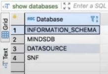
MindsDB comes with some built-in databases as follows:
INFORMATION_SCHEMA stores information about MindsDB,
MINDSDB stores metadata about the predictors and allows access to the created predictors as tables,
DATASOURCE for connecting to data or uploading files.
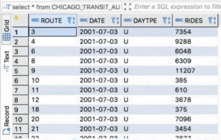
The SNF database is the database of the Chicago Transit Authority that we connected. It provides us with the training data. Let’s check it.
use snf;
SELECT *
FROM CHICAGO_TRANSIT_AUTHORITY.PUBLIC.CTA_BUS_RIDES_LATEST
LIMIT 100
The training data consists of the number of rides per bus route and day. For example, on 2001-07-03, there were 7354 rides on bus route 3.
Step 2: Training the Predictive Model
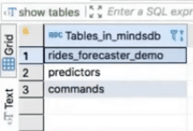
Let’s move on to the next step, which is training the predictive model. For that, we’ll use the MINDSDB database.
MINDSDB database comes with the predictors and commands tables. The predictors table lets us see the status of our predictive models. For example, assuming that we have already trained our predictive model for forecasting the number of rides, we’ll see the following.
SELECT name, status FROM
The process of training a predictive model using MindsDB is as simple as creating a view or a table.
CREATE MODEL rides_forecaster_demo FROM snf (
SELECT ROUTE, RIDES, DATE
FROM CHICAGO_TRANSIT_AUTHORITY.PUBLIC.CTA_BUS_RIDES_LATEST
WHERE DATE > '2020-01-01'
) PREDICT RIDES
ORDER BY DATE
GROUP BY ROUTE
WINDOW 10
HORIZON 7
Let’s discuss the statement above. We create a predictor table using the CREATE PREDICTOR statement and specifying the database from which the training data comes.
The code in yellow selects the filtered training data. After that, we use the PREDICT keyword to define the column whose data we want to forecast.
Next, there are standard SQL clauses, such as ORDER BY, GROUP BY, WINDOW, and HORIZON. We use the ORDER BY clause and the DATE column as its argument. By doing so, we emphasize that we deal with a time-series problem. We order the rows by date. The GROUP BY clause divides the data into partitions. Here, each of them relates to a particular bus route. We take into account just the last ten rows for every given prediction. Hence, we use WINDOW 10. To prepare the forecast of the number of bus rides for the next week, we define HORIZON 7.
Now, you can execute the CREATE PREDICTOR statement and wait until your predictive model is complete. The MINDSDB.PREDICTORS table stores its name as rides_forecaster_demo and its status as training. Once your predictive model is ready, the status changes to complete.
Step 3: Getting the Forecasts
We are ready to go to the last step, i.e., using the predictive model to get future data. One way is to query the rides_forecaster_demo predictive model directly. Another way is to join this predictive model table to the table with historical data before querying it.
We consider a time-series problem. Therefore, it is better to join our predictive model table to the table with historical data.
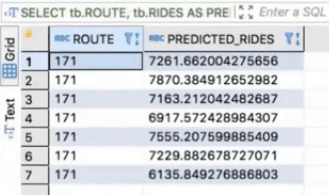
SELECT tb.ROUTE, tb.RIDES AS PREDICTED_RIDES
FROM snf.PUBLIC.CTA_BUS_RIDES_LATEST AS ta
JOIN mindsdb.rides_forecaster_demo AS tb
WHERE ta.ROUTE = "171" AND ta.DATE > LATEST
LIMIT 7
Let’s analyze it. We join the table that stores historical data (i.e., snf.PUBLIC.CTA_BUS_RIDES_LATEST) to our predictive model table (i.e., mindsdb.rides_forecaster_demo). The queried information is the route and the predicted number of rides per route. And the usage of the condition ta.DATE > LATEST (provided by MindsDB) ensures that we get the future number of rides per route.
Let’s run the query above to forecast the number of rides for route 171 in the next seven days.
Now we know the number of rides for route 171 in the next seven days. We could do it in the same way for all the other routes.
Thanks to the special SQL syntax that includes CREATE PREDICTOR, PREDICT, and > LATEST, MindsDB makes it straightforward to run predictors on our chosen data.
Now, let’s visualize our predictions.
Visualizing the Results using Apache Superset
Apache Superset is a modern, open-source data exploration and visualization platform designed for all data personas in an organization. Superset ships with a powerful SQL editor and a no-code chart builder experience. Superset ships with support for most SQL databases out of the box and over 50 visualization types.
You can connect to the Snowflake database or your MindsDB database that has a Snowflake connection within. Upon starting up your Superset workspace, your earlier defined database connection is ready to use! So you have access to the Chicago Transit Authority data, as well as to the predictions made by MindsDB.
Visualizing Data
The two data sets that we are relevant for visualization are the stops_by_route and forecasts data sets. The stops_by_route data set contains the exact location of each bus stop for each bus route. And the forecasts data set stores the actual and predicted number of rides, confidence interval, and lower and upper bounds of prediction, per route and timestamp.
Superset lets us visualize the stops_by_route data set as follows.
Every bus route has a different color. Also, there is volatility associated with each bus route. Let’s publish this chart to a new dashboard by clicking the +Save button, then switch to the Save as tab, and then type in “Routes Dashboard” in the Add to Dashboard field.
Now, let’s craft a time-series line chart to visualize actual vs predicted riders. Let’s look at the chart that presents the actual number of bus riders (in blue) and the predicted number of bus rides (in purple).
Predictions made by MindsDB closely resemble the actual data, except for a short time during March 2020 when the large-scale lockdowns took place. There we see a sudden drop in the number of bus rides. But MindsDB took some time to cope with this new reality and adjust its predictions.
Lastly, let’s add a data zoom to this chart for end-users to zoom in on specific date ranges. Click the Customize tab and then click Data Zoom to enable it. Then, click the + Save button and publish to the same “Routes Dashboard”.
Let’s head over to the dashboard now and customize it to make it more dynamic and explorable. Click Dashboards in the top nav bar and then select “Routes Dashboard” from the list of dashboards. You can rearrange the chart positions by clicking the pencil icon, dragging the corners of the chart objects, and then clicking Save.
Let’s add some dashboard filters to this dashboard so dashboard consumers can filter the charts down to specific bus routes and volatility values. Click the right arrow (->) to pop open the filter tray. Then select the pencil icon to start editing this dashboard’s filters. Create the following filters with appropriate filter names:
A Value filter on the route column from the forecasts table.
A Numerical range filter on the volatility column from the stops_by_route table.
Click Save to publish these filters.
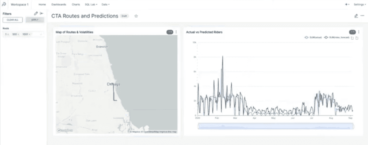
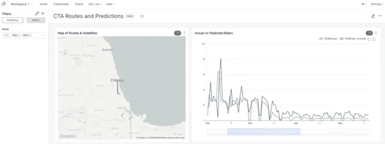
Let’s give these filters for a test ride! Use the routes filter to only show information for routes 1, 100, and 1001.
We could zoom in to see the time during the first large-scale lockdowns in March 2020. For these particular routes, the predictions made by MindsDB are not so far off.
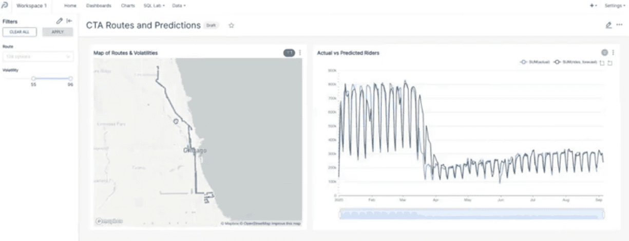
Now, let’s use our volatility filter to view only the routes with volatility values greater than 55.
MindsDB does a pretty good job as the actual and predicted number of rides are pretty close!
Conclusions: Powerful forecasting with MindsDB, Snowflake, and Superset
The combination of MindsDB and Snowflake covers all the phases of the ML lifecycle. And Superset helps you to visualize the data in any form of diagrams, charts, or dashboards.
MindsDB provides easy-to-use predictive models through AI Tables. You can create these predictive models using SQL statements and feeding the input data. Also, you can query them the same way you query a table. The easiest way to get started with Superset is with the free tier for Preset Cloud, a hassle-free and fully hosted cloud service for Superset.
Want to try it out yourself?
Bookmark MindsDB repository on GitHub
Access MindsDB via Docker, MindsDB’s Extension on Docker Desktop or AWS Marketplace.
Engage with the MindsDB community on Slack or GitHub to ask questions, share and express ideas and thoughts.
If this article was helpful, please give us a GitHub star here.
References:
¹ Data adapted from Algorithmia (2021). 2021 state of enterprise machine learning.

Start Building with MindsDB Today
Power your AI strategy with the leading AI data solution.
© 2025 All rights reserved by MindsDB.
Start Building with MindsDB Today
Power your AI strategy with the leading AI data solution.
© 2025 All rights reserved by MindsDB.

Start Building with MindsDB Today
Power your AI strategy with the leading
AI data solution.
© 2025 All rights reserved by MindsDB.